Getting Started with Machine Learning Using Keras

This blog post continues building on concepts introduced in Building Your First Neural Network series. It’s not necessary that you read those posts before reading this one. But it does explain more details on how a neural network learns, which we won’t really dive into in this post.

Machine Learning is a powerful technology. Today I’m going to show you how to get started with Keras, a Python Deep Learning Library.

Machine Learning Versus Deep Learning

What distinguishes machine learning and deep learning? Here’s how wikipedia defines both terms.

Machine learning is the study of computer algorithms that improve automatically through experience.

Wikipedia

Deep learning is part of a broader family of machine learning methods based on artificial neural networks with representation learning.

Wikipedia

Deep Learning is a type of Machine Learning where problems are solved using neural networks. Specifically, deep refers to the numerous layers that exist in neural networks.

The several networks that we’re going to build today are going to be very simple. So I wouldn’t really label them “deep networks”, but since this in a introductory blog post, it will do just fine.

MNIST Dataset

Today we’re going to create a couple neural networks that learn to recognize handwritten digits from the MNIST database. This database contains 70,000 handwritten examples broken into two groups, 60,000 training images and 10,000 test images.

Here is a sample of these digits.

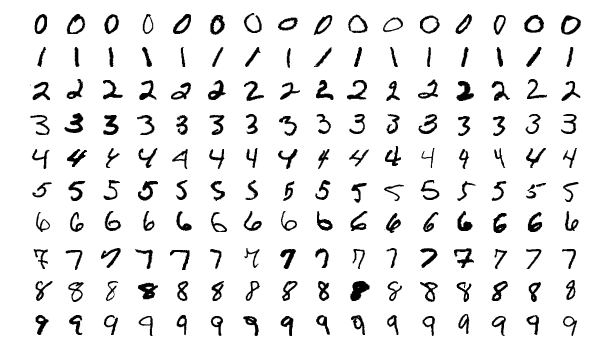
Each is a black and white photo that is 2828 pixels. This dataset is often considered the “Hello World” in machine learning.

Keras

What is Keras?

Keras is a high-level neural networks API, written in Python and capable of running on top of CNTK, or Theano. It was developed with a focus on enabling fast experimentation. Being able to go from idea to result with the least possible delay is key to doing good research.

keras.io

Keras is an API that facilitates communication with a machine learning library. Today we’ll be using a TensorFlow backend, but you could also run this using CNTK or Theano as mentioned above.

To run our examples we’ll be using Jupyter Lab, one of the easiest ways to get started writing and running python scripts.

I’m going to be using and building upon the mnist_mlp.py example contained in the keras github. If you’re curious of exploring keras more, I’d recommend checking those examples.

No Hidden Layer Neural Network

The first network that we’ll build is a network that has no hidden layers. It will have 784 input nodes, a dense layer in between that maps to 10 output nodes.

Here’s the code that will get everything setup to start learning.

Everything is relatively straightforward. A few things to note

• Lines 14-19 is us doing our data prep.
  • We resize our images from 2828 2d array to a 7841 array. This is a input format for our network.
• We clarify what type it is.
• Then we normalize the numbers by dividing by 255.
  • Our input image is a number from 0-255 indicating what shade of white/gray/black it is. 0 = white, 255 = black, everything in between is some shade of gray.
  • The difference between 0 and 255 is very large. Our network would encounter issues training on that range of data. Which is why we’re normalizing.
• Lines 22-23 converts the labels from single digit values to an array of length 10 where a 1 indicates which digit is correct.
  • 3 => [0, 0, 0, 1, 0, 0, 0, 0, 0, 0]
  • 6 => [0, 0, 0, 0, 0, 0, 1, 0, 0, 0]

Next we create our neural network, which I’ll refer to as both network and model in the remainder of this post.

Our model is sequential, which is a linear stack of layers. We have two layers, input and output.

Then we add a Dense layer to it, which has an input shape of 784, num_classes represents our output shape, and our activation is softmax.

Softmax ranks out output predictions and allows us to see how confident our neural network is in each answer.

We conclude this network by telling it how to train and evaluate itself.

Digging into the compile method a bit, the keras docs says it “Configures the model for training”. This is how we tell keras how we want our network to learn.

• We specify what method to use to calculate our loss.
  • The loss is how we quantify our how accurate/inaccurate our neural network is.
  • Here we are using categorical_crossentropy, another common one is mean_squared_error.
• Our optimizer helps our neural network know how to adjust our weights in order to learn.
  • When our network makes a prediction, measures it loss and then tries to update it’s weights, our optimizer tells our network how to move our weights to hopefully make a better prediction.
• And lastly our metrics, we’re testing for accuracy. How many of the images we can correctly guess.

What are our results when we train and test this network? Here is the final output from our model.

Test loss: 0.276
Test accuracy: 0.924

Our test accuracy is pretty good. Our network was able to learn how to recognize digits 92% of the time. Our loss is high, ideally our loss would be closer to 0.

For comparison, the neural network that we built by hand in our last article had an accuracy around 69%. It also trained a lot faster, 30 secs v 20 minutes.

Even though this was good, we can still do a lot better.

One Hidden Layer Neural Network

Next lets add one hidden layer into our network and see how it changes our accuracy.

A hidden layer is just a layer that is neither the input or output layer. ie, one of the middle layers.

• We’ve changed the output size of our first layer to now be 512, which is our hidden layer.
• We’ve also added a Dropout layer. A Dropout layer helps prevent our model from overfitting. Everytime we make a prediction we random turn off 20% (0.2) of our output layers. You’ll see this widely used in deep learning.
• Lastly we’ve added a relu activation to our first Dense layer. A relu layer is one way to add non-linearity to neural network.
  • A relu function works by changing all negative predictions to 0, any positive values remain unchanged.

Here are our results when using this network.

Test loss: 0.068
Test accuracy: 0.981

Both of our metrics vastly improved. Our hidden layer gave us greater ability to learn the patterns that exist in our digit data. Adding hidden layers tends to make overfitting easier, which is also why we added a dropout layer.

Two Hidden Layer Neural Network

One hidden layer was good, what happens if we add a second one?

Test loss: 0.0719
Test accuracy: 0.982

Our loss got bigger and our accuracy improved just a fraction. So in this case, adding a second hidden layer didn’t give us better predictive power.

Final Thoughts

Machine Learning is fun. Keras is a library that makes machine learning easier.

Even though our network learned to predict images with 98% accuracy, we can still do better. Convolutional Neural Networks (CCNs) is a different architecture that is especially helpful when dealing with images. But that’s something to explore in a different post!