Build Your First Neural Network: Part 1

This post is first in a series introducing neural networks. If you find this article helpful, you can continue onto Part 2 and Part 3.

Welcome to my first post about Machine Learning. Machine Learning is radically changing the types of tasks that computers can solve.

I’ve recently been exposing myself to it by reading Grokking Deep Learning by Andrew Task. I wanted to take some time today to explain the basics of machine learning, neural networks, then an example of a one neuron network.

The Basics

As with almost anything, starting with the basics and building a good foundation is critical for success. Machine Learning is no different. Some introductions start you with a machine learning library, or introduce the mathematics that drives neural networks. While those are helpful, I think starting with a simple example and building on that helps me learn faster.

First, lets talk a little about neurons and neural networks.

Artificial Neurons

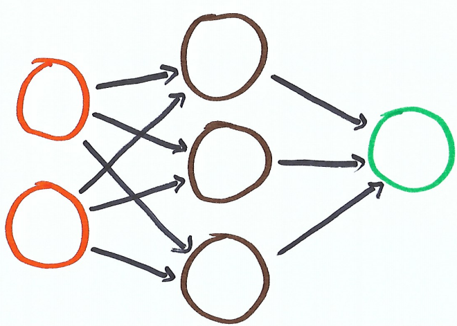
Both artificial neurons and neural networks are inspired by biology. The human brain is a biological neural network and has about 86 billion neurons.

Here is a diagram of a simple artificial neuron.

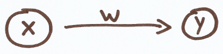
There’s an input (x), a weight (w) and an output (y). The formula for our simple neuron is y = xw.

If our weight is 0, then our output is 0.

If our weight is 1, then our output is the same as our input.

And if our weight is 2, then our output is double our input.

So far, pretty simply stuff. Even the definition for artificial neurons gets more complex, what artificial neurons do doesn’t change.

Artificial neurons take an input, apply some transformation, and output the result of that transformation. In this case, the weight (w) is the only thing affecting that transformation. (Formal definitions include a bias and an activation function)

I’m not sure if one neuron is technically considered a neural network (because network implies more than one), but our single neuron can still learn things, as we’re about to demonstrate.

Forward Propagation

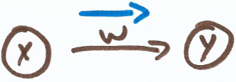
The flow of data through a neural network, from input, transformation and output, it is called forward propagation. Forward propagation is predicting. The output (y) of our neural network is the prediction.

Backpropagation

More importantly, we want our neural network to make accurate predictions. A neural network learns how to make accurate predictions during its training phase.

While training our neural network, its predictions are measured against the correct answer. If the prediction is wrong, we modify the neural network in the hope that in the future it makes a better prediction.

This process of updating the neural network is called backpropagation.

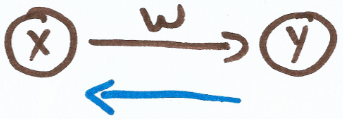
In our example, backpropagation will update the single weight. Hopefully allowing it to make a more accurate prediction in the future.

Our First Neural Network

Our first neural network is going to do something really simple, it’s going to learn how to output the input number.

So if we pass 1 as the input, it will predict 1. If we pass 2 as the input, it will predict 2.

Like I said, really simple. Our network will only consist of one neuron. Lets start small and build up the necessary parts of our network.

First we make a single prediction.

There’s an input, a weight and our pred, 0. This is the forward propagation part. We wanted it to predict the same number as our input, it didn’t do that.

That means our neuron has learning to do.

We know the answer is wrong, but how do we quantify that? We’ll introduce two new calculations, error and delta.

Our error tells us how far away we are from the right answer. We introduce goal_pred which is the answer that we’re looking for.

Since error is calculated via squaring, it’s always a positive number. This means its is a good measurement for how accurate our prediction is, but not a good indicator on how we should update our network to make better predictions.

That responsibility falls to delta.

Now delta will control how much we change our weight to hopefully get a better prediction in the future.

We now update our weight using delta.

Now our weight has changed to 1, which is the value we are looking for. The weight is multiplied by the input, and if the weight is 1 our prediction is correct.

Lets clean this up a bit, break out training and test data and condense our code. You’ll notice everything is still there, just rearranged a bit.

You’ll notice that this example “learns” how to return the input number and validates that using training data.

Congrats, you just wrote your first neural network.

Complicating Things

This is obviously a simplistic example, and has a lot of holes in it. For instance, if we switch our test and training data we don’t get the answer that we’re looking for.

This time our neural network wasn’t anywhere close to the answer. What happened? Our first example worked perfectly but our second was way off!

There are several problems, but the one we want to address now is our learning rate.

We use delta to tell us how much to update our weight. If our delta is big, our weight can change too much, we leads us to overshot our goal. Then every subsequent update takes us further and further away from our goal.

This is what happened in our example, we’re not converging to our optimal weight but diverging.

How can we control our learning rate? We’ll introduce another variable called alpha.

Notice our delta in our weight update (line 19) now is scaled by our alpha. We have to iterate through our training data 18 times, but eventually our weight converges onto our expected value (1).

Final Thoughts

This post just scratches the surface when it comes to machine learning. There’s so much more to learn and this simplistic example doesn’t do justice to the kinds of problems that can be solved with machine learning.

I’ll post more about it in the future, stay tuned.

If you found this helpful you can continue on to Part 2 of this series.