Build Your First Neural Network: Part 3
This post is the third in a series introducing you to neural networks. Feel free to read Part I and Part 2 before diving into this one.
The past two posts we’ve solved very basic formulas using neural networks. Now lets build a neural network to solve an actual problem. Our neural network will learn to recognize handwritten numbers.
The MNIST Dataset
The MNIST dataset is a classic “Hello World” type problem for machine learning.
The MNIST database of handwritten digits, available from this page, has a training set of 60,000 examples, and a test set of 10,000 examples. It is a subset of a larger set available from NIST. The digits have been size-normalized and centered in a fixed-size image. It is a good database for people who want to try learning techniques and pattern recognition methods on real-world data while spending minimal efforts on preprocessing and formatting.
These images are black and white 28x28 pixels of handwritten digits. Here are some samples from the dataset!
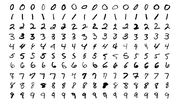
We’ll write a neural network to recognize this digits!
Expanding Our Understanding of Neural Networks
In Part 2 of this series, we wrote a simple 3-input 1-output neural network. Here is what that network looked like.
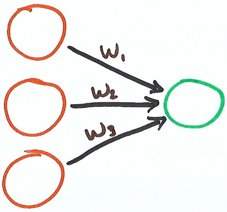
Each input (x) was multiplied by a weight (w), then summed together to get our output (y). Here is the formula for this neural network.
$$y = w_1 x_1 + w_2 x_2 + w_3 x_3$$
How do we go from a single output network to a multi output network? What if we needed to build a neural network that had both 3 inputs and 2 outputs?
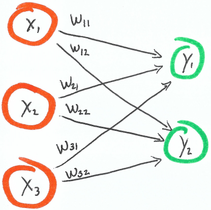
The number of inputs remain the same, but now we’ve added another output and 3 new weights.
You’ll see our weight notation changed. Now the weight identifies the two nodes it connects. The first subscript denotes which input its coming from and the second subscript denotes which output its going to.
$$w_{12} = \text{weight from}\, x_1\, \text{to}\, y_2$$
$$w_{31} = \text{weight from}\, x_3\, \text{to}\, y_1$$
We are building dense neural networks. A dense neural network is one that has a weight between every input and output node.
For building densely layered neural networks, 1. Determine how many inputs and outputs, 2. then create enough weights so there’s one weight between each input and output node.
To solve our MNIST problem, an image is our input, which is 2828 pixels. That means there’s 784 inputs. Our output guesses the digits 0-9, so we’ll need 10 outputs. Then for each input node, we’ll need a weight to map to each output node, which means we’ll have 7840 weights.
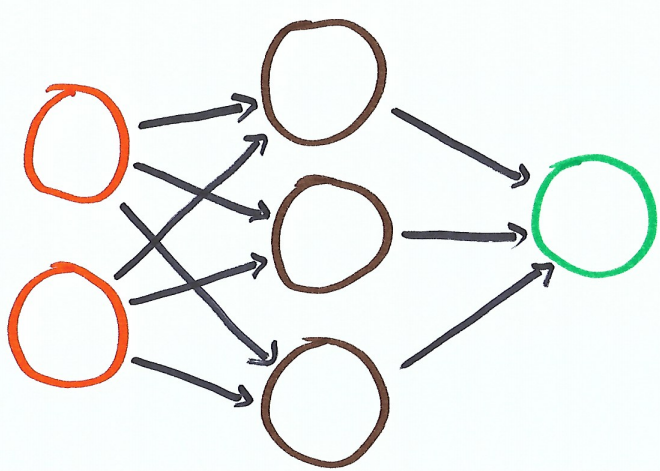
Visually, our neural network is going to look like this (minus the fact that I didn’t actually draw 784 inputs).
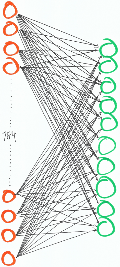
784 inputs, 10 outputs and a weight between each input and output.
Now lets get to coding that.
Obtaining and Normalizing Data
I’m using Jupyter Lab to run this code! As written this code will not work via the python cli.
To get our data we are going to use Keras and TensorFlow. Two popular machine learning libraries. We’ll only use them to get our data, so now that you know about them you can forget about them for the rest of this tutorial.
They automatically load our data for us.
You’ll notice that we have images and labels broken down into training and testing categories. We have 60,000 training examples and 10,000 testing examples.
The images are a 2828 array representing the grayscale (0-255) of the pixel at that location. The labels are a single digit indicating what that image is.
The next thing we’ll need to do is normalize our data. We’ll perform three normalizations for this problem.
- We’ll normalize the values in our pixel. Instead of the integer values 0-255, we want decimal values from 0-1. So we’re going to divide the images by 255.
- Then we want to reshape our images. Currently there in 2828 format, we’ll convert that into a single 784 length array to match our neural network input.
- We’ll convert labels into arrays. Labels are just a single number representing the given digit. Our prediction will be array of length 10, each value corresponding to the appropriate digit. So we need to perform the transformation.
Then here’s the code to train and test our images. Give it a look over and we’ll describe it more in the next section.
Training Phase
The training phase is our neural network learns to make accurate predictions. How does it learn?
For our neural network, we have our inputs, our weights and our outputs. If we want our outputs to change (learn to make better predictions), the only lever we have to move is our weights.
After each prediction we’ll calculate how much we need to move the weights to hopefully make a better prediction next time.
1st Training Image
Lets walk through our algorithm as it makes its first pass through our training data.
First we get our image and our label for our training data set. Then make a prediction given our image and our label. Which in our simple example boils down to the dot product between the image and the weights.
Here is the first prediction and correct label pair:
Prediction: [49.02 53.17 53.56 56.65 52.27 50.27 55.19 52.07 50.59 55.84]
Label: [0, 0, 0, 0, 0, 1, 0, 0, 0, 0]
Those predictions are pretty high compared to our expected output. It’s also wrong, the max value is 56.65 in index 3, meaning it guessed a 3. The label tells us the right answer is 4.
Since we initialized these weights randomly, it makes sense that they’re no where close to the right answer. So lets update our weights.
The next thing we do is calculate our error and our delta. error is a measurement of how far our prediction is away from the correct answer. As you’ll notice, it’s not actually used anywhere in our training. Usually this lets us, the humans, know how closely our neural network is to making accurate predictions. delta indicates how much we should change our weights to hopefully make a better prediction in the future.
Error: [2403 2827 2869 3209 2732 2428 3046 2712 2559 3118]
Delta: [49.02 53.17 53.56 56.65 52.27 49.27 55.19 52.07 50.59 55.84]
Since our prediction is really high, our delta is also high. This means we need to lower our weights quite a bit for our predictions to be closely to the right answer.
We then take the outer product of image and delta, this gives us an amount to update each individual weight.
Then we take our weight_deltas, scaled by our alpha and update our weights.
If you remember from last post, our alpha controls our learning rate. If we attempt to learn too quickly we’ll never converge to an accurate answer. If we learn too slowly it will take us forever to train. To pick this alpha I just tried a couple until one seemed to work. /shrug
101st Training Image
Now that we’ve trained on 100 images, lets see how our values have updated.
Here is our 101st prediction and correct label pair:
Prediction: [-1.18 -0.65  1.48 -1.11 0.25 -0.31 1.46  2.87  2.62  1.88]
Label: [0, 0, 0, 0, 0, 1, 0, 0, 0, 0]
But you’ll notice that our prediction has changed a lot in just 100 images. Instead of predictions in the 50 range, it’s outputting values between -1 and 2. That’s a small win!
Unfortunately this prediction is still incorrect. Our network predicted an 8, this image was labeled at 6. We still got some learning to do.
Lastly here is our error and delta:
Error: [1.39 0.42 2.21 1.24 0.06 1.73 2.14 8.25 6.89 3.54]
Delta: [-1.18 -0.65 1.48 -1.11 0.25 -1.31 1.46 2.87 2.62 1.88]
And after that we will complete the same weight updates as before.
Testing Phase
After we complete our training phase, we move onto our testing phase. In this phase we loop through our testing data, make a prediction and comparing against the label to know whether it was correct or not.
We can see how our learning improves with the number of images we train on.
- 0 training images : 1,256 / 10,000 = 12.56% correct
- 100 training images : 1,835 / 10,000 = 18.35% correct
- 1,000 training images : 3,129 / 10,000 = 31.29% correct
- 10,000 training images : 5,694 / 10,000 = 56.94% correct
- 20,000 training images : 5,709 / 10,000 = 57.09% correct
- 30,000 training images : 6,719 / 10,000 = 67.19% correct
- 40,000 training images : 5,751 / 10,000 = 57.61% correct
- 50,000 training images : 6,901 / 10,000 = 69.01% correct
- 60,000 training images : 6,928 / 10,000 = 69.28% correct
On my local machine, training 60,000 images took about 12 minutes.
With no training images, we guessed about 12% correct. Basically we’re just picking at random.
Then our network quickly improves as the training images scale to 10,000. Then from 10,000 to 60,000 training is a bit inconclusive. Sometimes it improves, while other times it takes a step back.
There are a lot of factors that go into how well a neural network can learn. Quality of data, training samples, how big the neural network is, how prone to overfitting your data is, on and on.
Given that, take a moment to appreciate what you accomplished. We built a neural network from scratch that correctly guessed almost 70% of our test images. That’s a good starting point.
Other machine learning algorithms can get 99% correct, so we definitely have a lot of room for improvement. Creating hidden layers, using CNNs, activation functions and biases are all things we can do to improve our algorithm. But don’t worry, we’ll get there all in due time.
Final Thoughts
Machine Learning and Neural Networks can be very powerful. Today’s post gives just a glimmer of what they can do. I hope you continue to play around with them and I’ll continue blogging about them!