Build Your First Neural Network: Part 2

A super dope neural network!!!

This post is the second in a series introducing you to neural networks. Feel free to read Part I before diving into this one, then read Part 3 afterwards.

Last week we talked about neural networks and showed how to use a simple neuron to learn a simple formula.

Today we’re going to build a slightly more complicated neural network to continue the learning process.

Our New Task

Today we’re going to build a neural network to learn this equation: $y = 0x_1 + x_2 + 2x_2$.

Yes, this is by no means ground breaking. No, we don’t need to use a neural network for this because we already have our equation. But it will be useful to demonstrate more concepts practicing on a problem that you already understand.

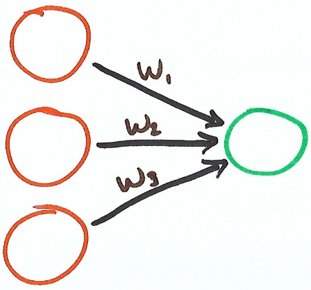
To do that we’ll be using a network with 3 inputs, 3 weights and 1 output.

Our neural network

As this is our first multi input network, lets take a step back and talk a bit about the math going on behind the scenes.

Math!!! (Everyone’s favorite subject)

As you learn more about machine learning, it’s important to understand the underlying mathematical principles. Lets talk about the different ways that we can mathematically model this neural network.

The first way is to describe our neural network is using a simple formula.

$$y = w_1 x_1 + w_2 x_2 + w_3 x_3$$

This formula can be simplified using summation.

$$y = \sum_{i=1}^3 w_i x_i $$

Then lastly we can use matrices and the dot product to represent our network.

$$\begin{bmatrix} x_1 & x_2 & x_3 \end{bmatrix} \cdot \begin{bmatrix} w_1 \\ w_2 \\ w_3 \end{bmatrix} = y$$

These three representations all describe the same thing, multiple the corresponding inputs and weights and sum them up.

Representing our neural network with matrices underscores how critical linear algebra is to the thorough understanding of neural networks. Neural networks use matrices and linear algebra a lot. If you aren’t very familiar with linear algebra, I would suggest brushing up on the basics.

Lets dive into the coding for our neural network. Like last article, we are going to write this neural network by hand.

Implementing our Neural Network

Lets start by defining our data and our neural network function.

For our trainingData, the first 3 elements represent our inputs and our fourth element represents our expected output.

Our alpha controls our learning rate, and I’ve chosen three values to start as our initial weights.

Our neural_network function performs the necessary calculations detailed in the above formulas. For each element in our inputs and weights matrices, multiple them and add them together.

Next thing we need to talk about is how we train our network. We need to perform the following steps:

Predict our value
Measure that value against the expected outcome
If our prediction is wrong, update our neural network in the attempt to predict more accurately in the future.

And we’re doing that! input corresponds to our formulas x values, weights corresponds to the w values, and pred corresponds to our y value.

Line 7 uses the dot product to determine our prediction.

On line 9, we calculate the mean squared error (MSE) to determine how far away from the answer our prediction is.

On line 10, we calculate delta for updating our weights.

And on line 14, we update each weight in turn depending on that specific weight’s input, our alpha and delta.

Here is a sampling of our output as we train our network. (I’ve rounded the values to make them easier to read)

0 - Input:[1, 2, 3], Pred:3.099, Goal:8, Error:24.01, Weight:[0.3, 0.23, 0.78]
0 - Input:[1, 1, 1], Pred:4.25, Goal:3, Error:1.562, Weight:[0.79, 1.21, 2.25]
0 - Input:[0, 1, 2], Pred:5.33, Goal:5, Error:0.11, Weight:[0.67, 1.09, 2.125]
0 - Input:[1, 2, 1], Pred:4.83, Goal:4, Error:0.68, Weight:[0.67, 1.05, 2.058]
0 - Input:[3, 1, 1], Pred:4.6, Goal:3, Error:2.59, Weight:[0.58, 0.8863, 1.98]
0 - Input:[4, 2, 2], Pred:5.48, Goal:6, Error:0.27, Weight:[0.09, 0.72, 1.815]
...
9 - Input:[1, 2, 3], Pred:8.04, Goal:8, Error:0.002, Weight:[0.01, 0.94, 2.05]
9 - Input:[1, 1, 1], Pred:2.98, Goal:3, Error:0.0004, Weight:[0.01, 0.9, 2.04]
9 - Input:[0, 1, 2], Pred:5.01, Goal:5, Error:0.0001, Weight:[0.012, 0.94, 2.04]
9 - Input:[1, 2, 1], Pred:3.92, Goal:4, Error:0.007, Weight:[0.012, 0.94, 2.03]
9 - Input:[3, 1, 1], Pred:3.05, Goal:3, Error:0.003, Weight:[0.02, 0.95, 2.04]
9 - Input:[4, 2, 2], Pred:5.98, Goal:6, Error:0.0003, Weight:[0.003, 0.95, 2.04]
...
50 - Input:[1, 2, 3], Pred:8.0001, Goal:8, Error:1.23e-08, Weight:[2.39-05, 0.999, 2.0001]
50 - Input:[1, 1, 1], Pred:2.999, Goal:3, Error:3.93-09, Weight:[1.27e-05, 0.999, 2.00009]
50 - Input:[0, 1, 2], Pred:5.0001, Goal:5, Error:1.32e-09, Weight:[1.89e-05, 0.999, 2.00009]
50 - Input:[1, 2, 1], Pred:3.999, Goal:4, Error:4.85e-08, Weight:[1.89e-05, 0.999, 2.00009]
50 - Input:[3, 1, 1], Pred:3.0001, Goal:3, Error:1.33e-08, Weight:[4.1e-05, 0.999, 2.0001]
50 - Input:[4, 2, 2], Pred:5.999, Goal:6, Error:1.28-09, Weight:[6.38e-06, 0.999, 2.0001]
...
235 - Input:[1, 2, 3], Pred:8.0, Goal:8, Error:0.0, Weight:[9.28e-17, 0.999, 2.0]
235 - Input:[1, 1, 1], Pred:3.0, Goal:3, Error:0.0, Weight:[9.28e-17, 0.999, 2.0]
235 - Input:[0, 1, 2], Pred:5.0, Goal:5, Error:0.0, Weight:[9.28e-17, 0.999, 2.0]
235 - Input:[1, 2, 1], Pred:4.0, Goal:4, Error:0.0, Weight:[9.28e-17, 0.999, 2.0]
235 - Input:[3, 1, 1], Pred:3.0, Goal:3, Error:0.0, Weight:[9.28e-17, 0.999, 2.0]
235 - Input:[4, 2, 2], Pred:6.0, Goal:6, Error:0.0, Weight:[9.28e-17, 0.999, 2.0]

You’ll see after 9 training iterations, the weights that we’ve learned are only several decimal places away from predicting the correct answer.

Then the rest of our training helps it adjust the weights to learn those last few decimal places.

You’ll also notice that on iteration 235, even though our prediction is correct, our weights are a fraction off from what the “right” answer is.

This underlies an important point of neural networks, we use our error (and delta) to inform us of when our learning has finished. If our error is zero (meaning the input and output align), we our network stops learning.

If for some reason a neural network finds a way to move our error to zero, it will stop learning even though it might not have found the optimal answer.

Playing with our Neural Network

Lets see what happens to our neural network when we modify it a bit. Lets change our starting weights to weights = [0.5337,0.0348,-0.3083] and see what happens. (again, rounded for presentation sake)

0 - Input:[1, 2, 3], Pred:-0.32, Goal:8, Error:69.25, Weight:[0.534, 0.035, -0.308]
0 - Input:[1, 1, 1], Pred:5.253, Goal:3, Error:5.077, Weight:[1.366, 1.699, 2.1881]
0 - Input:[0, 1, 2], Pred:5.399, Goal:5, Error:0.159, Weight:[1.141, 1.474, 1.9629]
0 - Input:[1, 2, 1], Pred:5.891, Goal:4, Error:3.577, Weight:[1.141, 1.432, 1.8829]
0 - Input:[3, 1, 1], Pred:5.603, Goal:3, Error:6.779, Weight:[0.951, 1.056, 1.6938]
0 - Input:[4, 2, 2], Pred:5.138, Goal:6, Error:0.742, Weight:[0.170, 0.795, 1.4335]
...
224 - Input:[1, 2, 3], Pred:8.0, Goal:8, Error:0.0, Weight:[6.89e-17, 0.999, 2.0]
224 - Input:[1, 1, 1], Pred:3.0, Goal:3, Error:0.0, Weight:[6.89e-17, 0.999, 2.0]
224 - Input:[0, 1, 2], Pred:5.0, Goal:5, Error:0.0, Weight:[6.89e-17, 0.999, 2.0]
224 - Input:[1, 2, 1], Pred:4.0, Goal:4, Error:0.0, Weight:[6.89e-17, 0.999, 2.0]
224 - Input:[3, 1, 1], Pred:3.0, Goal:3, Error:0.0, Weight:[6.89e-17, 0.999, 2.0]
224 - Input:[4, 2, 2], Pred:6.0, Goal:6, Error:0.0, Weight:[6.89e-17, 0.999, 2.0]

Very similar to our first set of weights, except its error converges to 0 in 11 fewer iterations.

Now, lets update our alpha to be 1 instead of 0.1.

0 - Input:[1, 2, 3], Pred:-0.32, Goal:8, Error:69.25, Weight:[0.534, 0.035, -0.308]
0 - Input:[1, 1, 1], Pred:50.18, Goal:3, Error:2226, Weight:[8.856, 16.678, 24.657]
0 - Input:[0, 1, 2], Pred:-75.57, Goal:5, Error:6492, Weight:[-38, -30, -22]
0 - Input:[1, 2, 1], Pred:200.42, Goal:4, Error:38581, Weight:[-38, 50, 138]
0 - Input:[3, 1, 1], Pred:-1104, Goal:3, Error:1227324, Weight:[-234, -342, -57]
0 - Input:[4, 2, 2], Pred:15985, Goal:6, Error:255340131, Weight:[3088, 765, 1050]

That very quickly goes to places nowhere close to the answer!!! Why is that?

When our network learns too quickly, it can have this back and forth behavior. It makes one prediction, sees that it’s wrong, the updates the weights too much in the opposite direction. That means the next prediction is even further from the right answer, forcing it to update the weights even more.

This behavior quickly spirals out of control. So much so that by the 35th iteration, after our error value is 9.748e+306 we encounter a python overflow error because our digits are too big.

That begs the question of what is an alpha that learns the appropriate amount? For the most part, just play with a couple different ones and pick the ones that actually converges on the answer.

Final Thoughts

I hope this part 2 was helpful in explaining more about how neural networks learn. For my next post, I’ll probably implement a neural network to try to learn how to accurately predict MNIST digits. Stay tuned.

Continue on to part 3 of this series to learn how to recognize handwritten digits.

I’m currently learning deep learning by reading through Grokking Deep Learning by Answer W. Trask. I highly recommend the book!!!